Some work (like programming) takes a lot of concentration, and I use noise-cancelling headphones to help me work productively in silence. But for other work (like doing business paperwork), I prefer to have quiet music in the background to help me stay focussed. Quiet background music is good for meditation or dozing, too. If you can’t fall asleep or completely clear your mind, zoning out to some music is the next best thing.

The best music for that is simple and repetitive — something nice enough to listen too, but not distracting, and okay to tune out of when needed. Computer game music is like that, by design, so there’s plenty of good background music out there. The harder problem is finding samples that play for more than a few minutes.

So I made loopx, a tool that takes a sample of music that loops a few times, and repeats the loop to make a long piece of music.

When you’re listening to the same music loop for a long time, even slight distortion becomes distracting. Making quality extended music audio out of real-world samples (and doing it fast enough) takes a bit of maths and computer science. About ten years ago I was doing digital signal processing (DSP) programming for industrial metering equipment, so this side project got me digging up some old theory again.

The high-level plan

It would be easy if we could just play the original music sample on repeat. But, in practice, most files we’ll have won’t be perfectly trimmed to the right loop length. Some tracks will also have some kind of intro before the loop, but even if they don’t, they’ll usually have some fade in and out.

loopx needs to analyse the music file to find the music loop data, and then construct a longer version by copying and splicing together pieces of the original.

By the way, the examples in this post use Beneath the Rabbit Holes by Jason Lavallee from the soundtrack of the FOSS platform game SuperTux. I looped it a couple of times and added silence and fade in/out to the ends.

Measuring the music loop length (or “period”)

If you don’t care about performance, estimating the period at which the music repeats itself is pretty straightforward. All you have to do is take two copies of the music side by side, and slide one copy along until you find an offset that makes the two copies match up again.

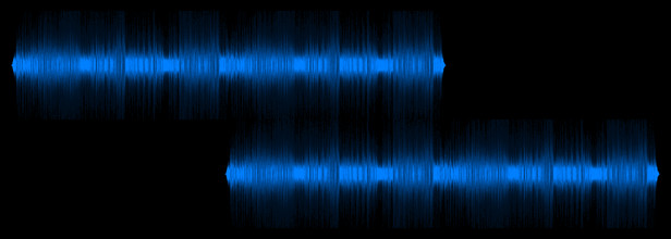
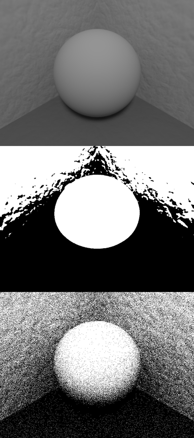
Now, if we could guarantee the music data would repeat exactly, there are many super-fast algorithms that could be used to help here (e.g., Rabin-Karp or suffix trees). However, even if we’re looking at computer-generated music, we can’t guarantee the loop will be exact for a variety of reasons like phase distortion (which will come up again later), dithering and sampling rate effects.

By the way, Chris Montgomery (who developed Ogg Vorbis) made an excellent presentation about the real-world issues (and non-issues) with digital audio. There’s a light-hearted video that’s about 20 minutes and definitely worth watching if you have any interest in this stuff. Before that, he also did an intro to the technical side of digital media if you want to start from the beginning.

If exact matching isn’t an option, we need to find a best fit instead, using one of the many vector similarity algorithms. The problem is that any good similarity algorithm will look at all the vector data and be $O(N)$ time at best. If we naïvely calculate that at every slide offset, finding the best fit will be $O(N^2)$ time. With over 40k samples for every second of music (multiplied by the number of channels), these vectors are way too big for that approach to be fast enough.

Thankfully, we can do it in $O(N \log N)$ time using the Fourier transform if we choose to use autocorrelation to find the best fit. Autocorrelation means taking the dot product at every offset, and with some normalisation that’s a bit like using cosine similarity.

The Fourier transform?

The Fourier transform is pretty famous in some parts of STEM, but not others. It’s used a lot in loopx, so here are some quick notes for those in the second group.

There are a couple of ways to think about and use the Fourier transform. The first is the down-to-earth way: it’s an algorithm that takes a signal and analyses the different frequencies in it. If you take Beethoven’s Symphony No. 9 in D minor, Op 125, Ode to Joy, and put it through a Fourier transform, you’ll get a signal with peaks that correspond to notes in the scale of D minor. The Fourier transform is reversible, so it allows manipulating signals in terms of frequency, too.

The second way to think of Fourier transforms is stratospherically abstract: the Fourier transform is a mapping between two vector spaces, often called the time domain and the frequency domain. It’s not just individual vectors that have mirror versions in the other domain. Operations on vectors and differential equations over vectors and so on can all be transformed, too. Often the version in one domain is simpler than the version in the other, making the Fourier transform a useful theoretical tool. In this case, it turns out that autocorrelation is very simple in the frequency domain.

The Fourier transform is used both ways in loopx. Because Fourier transforms represent most of the number crunching, loopx uses FFTW, a “do one thing really, really well” library for fast Fourier transform implementations.

Dealing with phase distortion

I had some false starts implementing loopx because of a practical difference between industrial signal processing and sound engineering: psychoacoustics. Our ears are basically an array of sensors tuned to different frequencies. That’s it. Suppose you play two tones into your ears, with different phases (i.e., they’re shifted in time relatively to each other). You literally can’t hear the difference because there’s no wiring between the ears and the brain carrying that information.

Sure, if you play several frequencies at once, phase differences can interact in ways that are audible, but phase matters less overall. A sound engineer who has to make a choice between phase distortion and some other kind of distortion will tend to favour phase distortion because it’s less noticeable. Phase distortion is usually simple and consistent, but phase distortion from popular lossy compression standards like MP3 and Ogg Vorbis seems to be more complicated.

Basically, when you zoom right into the audio data, any algorithmic approach that’s sensitive to the precise timing of features is hopeless. Because audio files are designed for phase-insensitve ears, I had to make my algorithms phase-insensitive too to get any kind of robustness. That’s probably not news to anyone with real audio engineering experience, but it was a bit of an, “Oh,” moment for someone like me coming from metering equipment DSP.

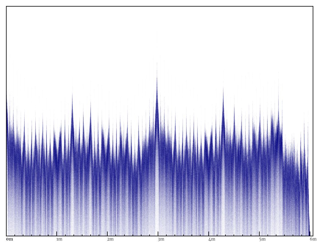
I ended up using spectrograms a lot. They’re 2D heatmaps in which one axis represents time, and the other axis represents frequency. The example below shows how they make high-level music features much more recognisable, without having to deal with low-level issues like phase. (If you’re curious, you can see a 7833x192 spectrogram of both channels of the whole track.)

The Fourier transform does most of the work of getting frequency information out of music, but a bit more is needed to get a useful spectrogram. The Fourier transform works over the whole input, so instead of one transformation, we need to do transformations of overlapping windows running along the input. Each windowed transformation turns into a single frame of the spectrogram after a bit of postprocessing. The Fourier transform uses a linear frequency scale, which isn’t natural for music (every 8th white key on a piano has double the pitch), so frequencies get binned according to a Mel scale (designed to approximate human pitch perception). After that, the total energy for each frequency gets log-transformed (again, to match human perception). This article describes the steps in detail (ignore the final DCT step).

Finding the loop zone

Remember that the music sample will likely have some intro and outro? Before doing more processing, loopx needs to find the section of the music sample that actually loops (what’s called the “loop zone” in the code). It’s easy in principle: scan along the music sample and check if it matches up with the music one period ahead. The loop zone is assumed to be the longest stretch of music that matches (plus the one period at the end). Processing the spectrogram of the music, instead of the raw signal itself, turned out to be more robust.

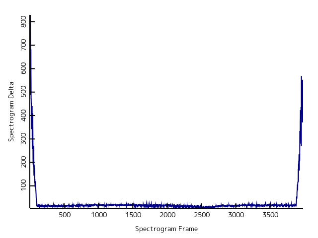
A human can eyeball a plot like the one above and see where the intro and outro are. However, the error thresholds for “match” and “mismatch” vary depending on the sample quality and how accurate the original period estimate are, so finding a reliable computer algorithm is more complicated. There are statistical techniques for solving this problem (like Otsu’s method), but loopx just exploits the assumption that a loop zone exists, and figures out thresholds based on low-error sections of the plot. A variant of Schmitt triggering is used to get a good separation between the loop zone and the rest.

Refining the period estimate

Autocorrelation is pretty good for estimating the period length, but a long intro or outro can pull the estimate either way. Knowing the loop zone lets us refine the estimate: any recognisable feature (like a chord change or drum beat) inside the loop zone will repeat one period before or after. If we find a pair of distinctive features, we can measure the difference to get an accurate estimate of the period.

loopx finds the strongest features in the music using a novelty curve — which is just the difference between one spectrogram frame and the next. Any change (a beat, a note, a change of key) will cause a spike in this curve, and the biggest spikes are taken as points of interest. Instead of trying to find the exact position of music features (which would be fragile), loopx just takes the region around a point of interest and its period-shifted pair, and uses cross-correlation to find the shift that makes them best match (just like the autocorrelation, but between two signals). For robustness, shifts are calculated for a bunch of points and the median is used to correct the period. The median is better than the average because each single-point correction estimate is either highly accurate alone or way off because something went wrong.

Extending the music

The loop zone has the useful property that jumping back or forward a multiple of the music period keeps the music playing uninterrupted, as long as playback stays within the loop zone. This is the essence of how loopx extends music. To make a long output, loopx copies music data from the beginning until it hits the end of the loop zone. Then it jumps back as many periods as it can (staying inside the loop zone) and keeps repeating copies like that until it has output enough data. Then it just keeps copying to the end.

That sounds simple, but if you’ve ever tried it you’ll know there’s one more problem. Most music is made of smooth waves. If you just cut music up in arbitrary places and concatenate the pieces together, you get big jumps in the wave signal that turn into jarring popping sounds when played back as an analogue signal. When I’ve done this by hand, I’ve tried to minimise this distortion by making the curve as continuous as possible. For example, I might find a place in the first fragment of audio where the signal crosses the zero line going down, and I’ll try to match it up with a place in the second fragment that’s also crossing zero going down. That avoids a loud pop, but it’s not perfect.

An alternative that’s actually easier to implement in code is a minimum-error match. Suppose you’re splicing signal A to signal B, and you want to evaluate how good the splice is. You can take some signal near the splice point and compare it to what the signal would have been if signal A had kept playing. Simply substracting and summing the squares gives a reasonable measure of quality. I also tried filtering the errors before squaring and summing because distortion below 20Hz and above 20kHz isn’t as bad as distortion inside normal human hearing range. This approach improved the splices a lot, but it wasn’t reliable at making them seamless. I don’t have super hearing ability, but the splices got jarring when listening to a long track with headphones in a quiet room.

Once again, the spectral approach was more robust. Calculating the spectrum around the splice and comparing it to the spectrum around the original signal is a useful way to measure splice quality. The pop sound of a broken audio signal appears as an obvious burst of noise across most of the spectrum. Even better, because the spectrum is designed to reflect human hearing, it also catches any other annoying effects, like a blip caused by a bad splice right on the edge of a drum beat. Anything that’s obvious to a human will be obvious in the spectrogram.

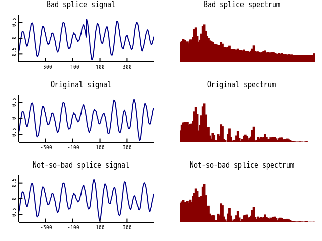
There are multiple splice points that need to be made seamless. The simple approach to optimising them is a greedy one: just process each splice point in order and take the best splice found locally. However, loopx also tries to maintain the music loop length as best as possible, which means each splice point will depend on the splicing decisions made earlier. That means later splices can be forced to be worse because of overeager decisions made earlier.

Now, I admit this might be getting into anal retentive territory, but I wasn’t totally happy with about %5 of the tracks I tested, and I wanted a tool that could reliably make music better than my hearing (assuming quality input data). So I switched to optimising the splices using Dijkstra’s algorithm. Normally Dijkstra is thought of as an algorithm for figuring out the shortest path from start to finish using available path segments. In this case, I’m finding the least distortion series of copies to get from an empty output audio file to one that’s the target length, using spliced segments of the input file. Abstractly, it’s the same problem. I also calculate cost a little differently. In normal path finding, the path cost is the sum of the segment costs. However, total distortion isn’t the best measure for loopx. I don’t care if Dijkstra’s algorithm can make an almost-perfect splice perfect if it means making an annoying splice worse. So, loopx finds the copy plan with the least worst-case distortion level. That’s no problem because Dijkstra’s algorithm works just as well finding min-max as it does finding min-sum (abstractly, it just needs paths to be evaluated in a way that’s a total ordering and never improves when another segment is added).

Enjoying the music

It’s rare for any of my hobby programming projects to actually be useful at all to my everyday life away from computers, but I’ve already found multiple uses for background music generated by loopx. As usual, the full source is available on GitLab.